[Draft] Bag of Tricks for Image Classification with Convolutional Neural Networks

Refinements play an important role in deep learning workflow. These includes changes in loss functions, data preprocessing and optimization methods. These refinements improve the model accuracy by a few percentage (which is quite significant if you were to compare the state-of-the-art models in a specific category, for example image captioning) but they are typically not covered in details in the papers. In this paper, we can learn different tricks that could be applied to our own model and their impacts.

In the following sections, I will break down the discussion into different sections. These sections will either include discussion on individual chapter or a group of chapters.

Introduction

Examine collection of training and model architecture refinements

• minor tricks, for example: modifying stride
• adjusting learning rate schedule Together they make big difference

These tricks will be evaluated on multiple network and impact are reported to the final model accuracy

Advantage of their Tricks

• Can be generalize to other networks (inception and mobilenet) and other datasets (Place365)
• Bring better transfer learning performance in other applications such as object detection and semantic segmentation

Training procedure

The template that the network uses is mini-batch stochastic gradient descent. Author argued that functions and hyper-parameters in the baseline algo can be implemented in different ways

Baseline training procedure

The preprocessing pipelines between training and validation are different

During training:

1. randomly sample an image and decode it into 32-bit raw values in [0,255]
2. crop a rectangular region whose aspect ratio is randomly sampled in [3/4,4/3] and area randomly sampled in [8%, 100%], then resize the cropped image into 224x224
3. Flip horizontally with 0.5 probability
4. Scale hue, saturation, and brightness with coefficients uniformly drawn from [0.6,1.4]
5. Add PCA noise with a coefficient sampled from a normal distribution $N$(0,0.1)
6. Normalize RGB channels by subtracting the pixels with 123.68, 116.779, 103.939 and dividing by 58.393, 57.12, 57.375

During validation:

1. Resize each image’s shorted edge to 256 pixels while keeping its aspect ratio.
2. Crop a 224x224 region in the center
3. Normalize RGB channels the same way as step.no 6 for training data

Weights initialization:

1. Both convolutional and fully-connected layers are initialized with Xavier algorithm
2. In particular, parameters are set to random values uniformly drawn from [-a, a], where $a = \sqrt{6/(d_{in}-d_{out})}$. $d_{in}$ and $d_{out}$ are the input and output channel sizes, respectively.
3. All biases are initilized to 0
4. For batch normalization layers, $\gamma$ vectors are initilized to 1 and $\beta$ vectors to 0.

Optimizer:

1. Nesterov Accelerated Gradient (NAG) descent is used for training.
2. Each model trained for 120 epoch on 8 Nvidia V100 GPUs, batch_size set to 256.
3. Learning rate is initialized to 0.1 and divided by 10 at the 30th, 60th, and 90th epochs.

What is Nesterov Accelerated Gradient (NAG) Descent?
It is important to understand NAG Descent here before we discuss about other improvements on the model. Momentum based Gradient Descent solves the problems of Vanilla Gradient Descent in such a way that it doesn’t get stuck in the gentle region. The way it does is aggregate previous updates to learn the weights with a larger step.
However, it tends to oscillate in the valley region before going down to the trough. This leads to more redundant iterations in order to get the optimum point for the training. To understand more, I will cover this in another blog post. Stay tuned!

The experiments were done with three CNNs: ResNet-50, Inception-V3 (images are resized into 299x299), and MobileNet. They tested them on ISLVRC2012 dataset, which contains 1.3 million images for training and 1000 classes.

Validation accuracy of reference implementations and the author’s model baseline

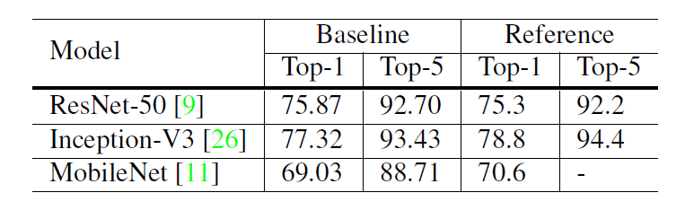
As shown above, only ResNet-50 shows better results than the reference’s one while the other models perform slightly poorer than its reference counterpart.

Efficient Training

During the early stage of GPU development, developers will need to make a decision between accuracy and speed. However, due to recent advancement in high-performance computing, it is now more efficient to use lower numerical precision (To understand the benefit of lower numerical precision, check out this post) and larger batch sizes during training.

However, there are some reports(here and here, the second link includes answer from Ian Goodfellow) that critisized on training with larger batch size. So, what techniques we can use to make full advantage of these two constraints without degrading our model accuracy?

Large-batch Training

The advantages of using large-batch training is two-fold: increase parallelism and decrease communication costs. However, every coin has two sides. The cost of using it is slower training as convergence rate tends to slow down when the batch size increases. In the similar context, if we fix the number of epochs for two different models: one trains with large batch size and the other trains with single batch size at a single time, we would expect the former to end up with degraded validation accuracy as compared to the latter. Below we will discuss 4 heuristics to solve the problem.

• Linear scaling learning rate Increasing the batch size can reduce its variance (or noise in the gradient). Goyal et al. pointed out that linearly increasing the learning rate with larger batch size works empirically for ResNet-50 training. The author suggests that we can choose the initial learning rate by calculating this equation $0.1 \times \frac{b}{256}$ if we follow He et al. to choose 0.1 as initial learning rate.

• Learning rate warmup Using large learning rate may result in numerical instability at the start of the training. Goyal et al. suggests a gradual warmup strategy that increases the learning rate from 0 to the initial learning rate linearly. In other words, we can set the learning rate to $\frac{i\eta}{m}$, where n is the initial learning rate at batch $i$, $1 \leq i \leq m$.

• Zero $\gamma$ The output of the residual block is equal to $x + block(x)$. Inside of the block is convolutional layers. For some variant of residual block, the last layer could be a batch normalizaton (BN) layer. The last operation of BN layer is scale transformation $\gamma\hat{x}+\beta$ and both $\gamma$ and $\beta$ are learnable parameters whose elements are initialized to 1s and 0s, respectively. The author suggests that we should set $\gamma$ to be zero so that the network has less parameters to learn and easier to train.

• No bias decay Weight decay is often applied to both weights and bias (equivalent to applying L2 regularization). However, Jia et al. suggests that we should apply weight decay to the weights in convolution and fully-connected layers and left biases and $\gamma$ and $\beta$ in BN layers unregularized.

Low-precision training

Comparison of the training time and validation accuracy for ResNet-50 between the baseline (BS=256 with FP32) and a more hardware efficient setting (BS=1024 with FP16)

The training speed is accelerated by 2 or 3 times after switching from FP32 to FP16 on Nvidia V100. See figure above. However, the best practice is to store all parameters and activations in FP16 and use FP16 to computer the gradients. At the same time, all parameters have an copy in FP32 for parameter updating.

Model Tweaks

Minor adjustment to the network architecture barely changes the computational complexity. However, it may get you non-negligible effect on the model accuracy. In the following sections, we will use ResNet as an example to discuss about a few tweaks to make a better model.

Original ResNet introduced in He et al..

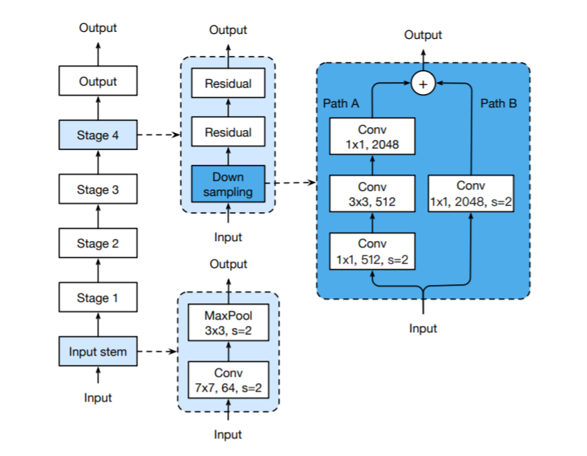
The figure above illustrates the architecture of ResNet-50. The author points out a few tweaks that focuses on the input stem and down-sampling block.

ResNet Tweaks.

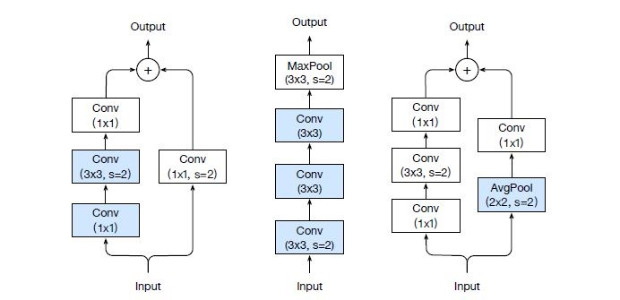
1. ResNet-B modifies the first two Conv layers in Path A. The motivation is to solve the loss of information due to the stride of 2 in the first Conv layer.
2. ResNet-C replaces the 7x7 convolution layers as its inherently much more expensive that 3x3 convolution layers in term of the computational cost. This concept originates from Inception-V2.
3. ResNet-D removes the stride of 2 in the Conv layer appeared in Path B. At the same time, it introduces a 2x2 average pooling layer with a stride of 2 and it works well empirically.

Training Refinements

There are four training refinements discussed here:

Cosine Learning Rate Decay