![MNIST Classifier with Pytorch [Part I]](https://cdn-images-1.medium.com/max/2600/1*aqNgmfyBIStLrf9k7d9cng.jpeg)

MNIST Classifier with Pytorch [Part I]
I am doing a revision on how to build neural network with PyTorch. To do so I am taking Udacity’s online lesson on Intro to Deep Learning with PyTorch. This course introduces many important models such as CNN and RNN using PyTorch. In the subsequent posts, I will try to summarize important points that I have learnt in the course.
Prerequisite
For those who have learnt fundamental deep learning concepts should not find any difficulties to follow. However, if you are a fresh new beginner in this field, I would strongly encourage you to go through Andrew Ng’s Deep Learning Specialization on Coursera before reading this entire post series.
What is MNIST Dataset?
MNIST consists of greyscale handwritten digits ranging from 0 to 9. Each image is 28 x 28 pixels.

What is PyTorch?
As its name implies, PyTorch is a Python-based scientific computing package. It allows developers to compute high-dimensional data using tensor with strong GPU acceleration support. One of the advantages over Tensorflow is PyTorch avoids static graphs. This allows developers to change the network behavior on the fly.
I was reluctant to use PyTorch when I first started learning deep learning is because of it poor production support. However, recent release of PyTorch 1.0 has overcome the challenges. The merge between PyTorch and Caffe2 allows researchers to move seemlessly from research to production without worries about migration issue.
Overall speaking, it’s always good to learn both Tensorflow and PyTorch as these two frameworks are designed by the two giant companies which focus heavily on Deep Learning development. There is no reason to choose either side especially for someone who wishes to make their models reachable to the community.
Basic Workflow
In this section, we will discuss about the basic workflow of classifying image using PyTorch.
Import Library
To build the model, we need the tools. We first import the libraries which are needed for our model.
import torch
from torch import nn, optim # Sets of preset layers and optimizers
import torch.nn.functional as F # Sets of functions such as ReLU
from torchvision import datasets, transforms # Popular datasets, architectures and common image transformations for computer vision
Transfrom Dataset
Before we download the data, we will need to specify how we want to transform our dataset. This is a bit different from the Keras’s workflow; where we import the dataset then transform the data into the format that we want.
There are two basic transformations that is required for this dataset: turn the raw data into tensor and normalize the data with mean and standard deviation.
As in the example below, we passed 0.5 to both parameters mean and std so that the resulted image could be in the range [-1,1]. See the explanation here. Normalization is an important step towards a faster and efficient deep learning model.
Neural network learns how to predict the data by updating its parameters. During training, some features with larger numerical values tend to be assigned with larger parameters. By doing so, we miss the opportunity to learn from other features that could have significant impact on the prediction. Therefore, we need normalization to set every features at the same “starting line” and let the network to decide which feature is important.
tranform = tranforms.Compose([transforms.ToTensor(),
                              transforms.Normalize((0.5,0.5,0.5),(0.5,0.5,0.5))])
Download Training Dataset
To download the dataset, we use torchvision dataset library.
trainset = datasets.MNIST('~/MNIST_data/', download=True, train=True, transform=transform)
Load Dataset
To load the dataset efficiently, we need to utilize the dataloader function.
Normally, when we load data from the dataset, we will naively use forloop to iterate over data. By doing so we are refraining ourselves from:
- Batching the data. Retrieving dataset by batches for mini-batch training
- Shuffling the data. To allow model see different set of training batch in every iteration. This helps to avoid biased estimate. See the explanation on why its important to shuffle data.
- Load the data in parallel using
multiprocessingworkers.
Therefore, we use dataloader to solve the abovementioned issues.
trainloader = torch.utils.data.DataLoader(trainset, batch_size=64, shuffle=True)
Build a simple feed-forward network
There are different ways to build model using PyTorch. One is to define a class and the other is to use nn.Sequential. Both ways should lead to the same result. However, defining a class could give you more flexibility as custom functions can be introduced in the forward function.
Model are usually defined by subclassing torch.nn.Module and operations are defined by using torch.nn.functional. We first specify the model’s parameters and then specify how they are applied to the inputs. torch.nn.functional usually deals with operations without trainable parameters.
In the following example, we will show two different approaches. You can whichever way you like to build your model.
Load images and define loss function
# Get data in a batch of 64 images and their corresponding labels
images, labels = next(iter(trainloader))

# Flatten every images to a single column
images = images.view(images.shape[0],-1)

# Define the loss
criterion = nn.CrossEntropyLoss()
[Option 1] Model defined using nn.Sequential
model = nn.Sequential(nn.Linear(784, 128),
                      nn.ReLU(),
                      nn.Linear(128,64),
                      nn.ReLU(),
                      nn.Linear(64,10))
[Option 2] Model defined using class
class SimpleNetwork(nn.Module):
    def __init__(self):
        super().__init__()

        self.hidden_1 = nn.Linear(784,128)
        self.hidden_2 = nn.Linear(128,64)
        self.output = nn.Linear(64,10)

    def forward(self,x):
        x = F.relu(self.hidden_1(x))
        x = F.relu(self.hidden_2(x))
        y_pred = self.output(x)
        return y_pred

# Initialize the network
model = SimpleNetwork();
Predict labels and calculate loss
# Get the prediction for each images
logits = model(images)

# Calculate the loss
loss = criterion(logits, labels)
Here we split the steps into four different sections for clarity:
- Load images and define loss function
- Here we need to load the images and their corresponding labels so that we can put them through the model and evaluate the result. Loss function requires two input: prediction and true labels.
- nn.Sequential and class implementations
- As mentioned before, although their implementations are different, but both ways should lead to the same result.
- Predict labels and calculate loss
- We pass the images to the model and we receive the predictions. After that, we compare the predicted output with the true label.
It is important to understand the loss function here. We use CrossEntropyLoss in our model. It is a loss that combines both LogSoftMax and NLLLoss (Negative Log Likelihood) in one single class.
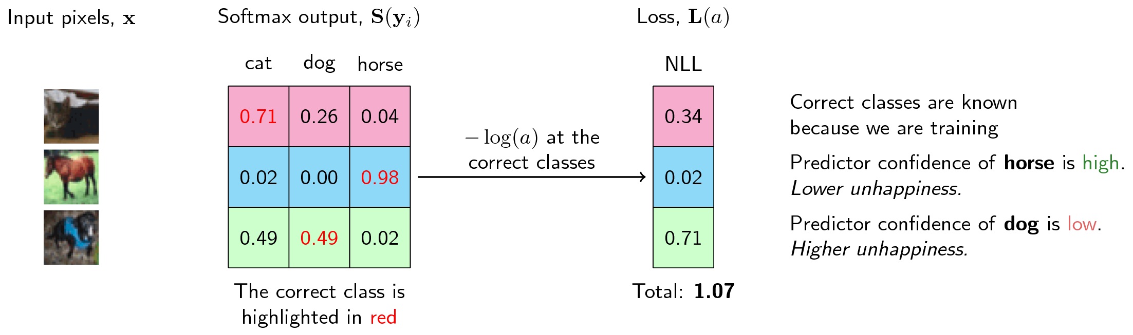
The loss function assigns low value to model when the correct label is assigned with higher confidence. If the model classifies incorrectly, higher penalty will be imposed.
Backpropagation
To perform backpropagation, we need to use a Torch module autograd for automatically calculating the gradients of tensors. By using this module, we can calculate the gradient of the loss w.r.t. our parameters.
We can also turn off gradients for a block of code with torch.no_grad() content:
# x requires gradient calculation
x = torch.zeros(10,10, requires_grad=True)

# y does not require gradient calculation
with torch.no_grad():
    y = x * 2
When we do backpropagation, what’s happening is we are trying to optimize the model by locating the weights that result in the lowest possible loss. So we need to do a backward pass starting from the loss to find the gradients.
loss.backward()
Optimizer
To update the weights with the gradients, we will need an optimizer. PyTorch provides an optim package to provide various optimization gradients. For example, we can use Stochastic Gradient Descent with optim.SGD.
# Optimizers require parameters to optimize and a learning rate
optimizer = optim.SGD(model.parameters(), lr=0.01)
To recap, the general process with PyTorch:
- Make forward pass through the network
- Calculate loss with the network output
- Calculate gradients by using
loss.backward()to perform backpropagation - Update weights using optimizer
Important
It’s important to note that before we can update our weights, we need to use optimizer.zero_grad() to zero the gradients on each training pass. This is because in PyTorch the gradients are accumulated from previous training batches.
Overall Workflow Recap (for only one training step)
images, labels = next(iter(trainloader)) # Extract images

optimizer.zero_grad() # Clear gradients

output = model.forward(images) # Forward pass

loss = criterion(output, labels) # Calculate loss

loss.backward() # Backward pass

optimizer.step() # Optimize weights
Conclusion
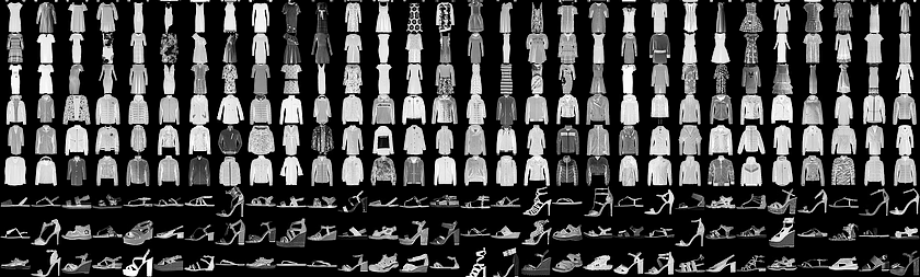
So we have a working MNIST digits classifier! To conclude, we have learnt the workflow of building a simple classifier using PyTorch and the basic components that can provide additional “power” for us to efficiently construct the network. Next, we will build another simple classifier to classify the clothing images. Fashion-MNIST dataset is more complex than MNIST so it can kind of like resemble the actual real-world problem.
Leave a comment